Logistic(; alpha = 0.01, ni = 1000)

Logistic Regression classifier.

This struct learns classifiers using multi class softmax. Parameter α indicates the learning rate, and ni indicates the number of learnings.

Example

julia> model = Logistic(alpha = 0.1)
Logistic(0.1, 1000, Matrix{Float64}(undef, 0, 0))

julia> fit!(model, x, ct)
3×3 Matrix{Float64}:
  1.80736  1.64037  -0.447735
 -1.27053  1.70026   2.57027
  4.84966 -0.473835 -1.37582

julia> println(predict(model, x))
[1, 1, 1, 1, 1, 1, 1, 1, 1, 1, 1, 1, 1, 3, 3, 3, 3, 3, 3, 3, 3, 3, 3, 3, 3, 3, 3, 3, 3, 3, 3, 3, 3, 3, 3, 3, 3]

SVC(; alpha=0.01, ni=1000)

Support Vector Machine Classifier.

This struct learns classifiers using One-Vs-Rest. One-Vs-Rest generates two-class classifiers divided into one class and the other classes using Logistic Regression, adopting the most likely one among all classifiers.

Parameter α indicates the learning rate, and ni indicates the number of learnings.

Example

julia> model = SVC()
SVC(0.01, 1000, Logistic[])

julia> fit!(model, ct)
3-element Vector{Logistic}:
 Logistic(0.01, 1000, [0.8116709490679518 1.188329050932049; 1.7228257190036231 0.2771742809963788; -0.1519960725403138 2.1519960725403116])
 Logistic(0.01, 1000, [0.9863693439936144 1.0136306560063886; 0.8838433946106077 1.11615660538939; 1.4431044559203794 0.5568955440796174])
 Logistic(0.01, 1000, [1.262510641510418 0.7374893584895849; 0.5242383002319192 1.4757616997680822; 1.864635796779504 0.135364203220495])

julia> println(predict(model, x))
[1, 1, 1, 1, 1, 1, 1, 1, 1, 1, 1, 1, 1, 3, 3, 3, 3, 3, 3, 3, 3, 3, 3, 3, 3, 3, 3, 3, 3, 3, 3, 3, 3, 3, 3, 3, 3]

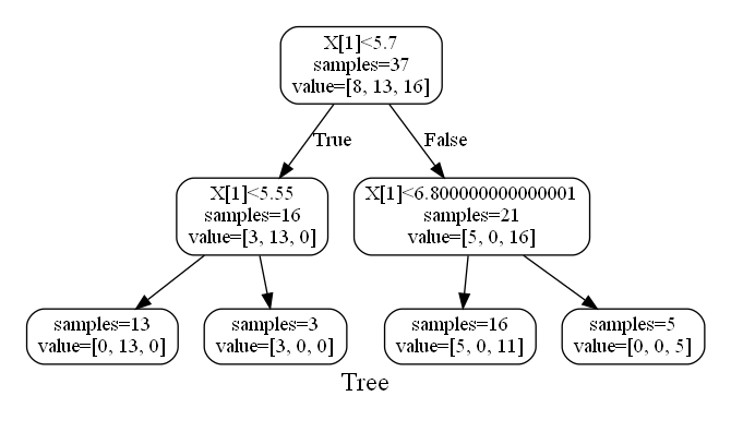
DecisionTree(; alpha = 0.01)

Normal DecisionTree. alpha specify the complexity of the model. If it's small, it's complicated, and if it's big, it's simple.

Example

julia> tree = DecisionTree()
DecisionTree(0.01, Dict{Any, Any}(), Any[])

julia> fit!(tree, x, t)
Dict{String, Any} with 5 entries:
  "left"        => Dict{String, Any}("left"=>Dict{String, Union{Nothing, Vector…
  "class_count" => [8, 13, 16]
  "threshold"   => 5.7
  "right"       => Dict{String, Any}("left"=>Dict{String, Union{Nothing, Vector…
  "feature_id"  => 1

julia> println(predict(tree, x))
[0, 0, 0, 0, 0, 0, 0, 0, 0, 0, 0, 0, 0, 2, 2, 2, 2, 1, 2, 1, 1, 2, 2, 2, 2, 2, 2, 2, 2, 2, 2, 2, 2, 2, 2, 2, 2]

RandomForest(nt; alpha = 0.01)

RandomForest Model. nt is the number of trees, and alpha is the same as alpha in DecisionTree.

Example

julia> model = RandomForest(10)
RandomForest(0.01, 10, DecisionTree[], Vector{Any}[], #undef)

julia> fit!(model, x, t)
10×1 Matrix{Int64}:
 1
 2
 2
 2
 2
 1
 1
 1
 1
 1

julia> println(predict(model, x))
Any[0, 0, 0, 0, 0, 0, 0, 0, 0, 0, 0, 0, 0, 2, 1, 2, 2, 1, 2, 2, 1, 2, 2, 2, 2, 2, 2, 2, 2, 2, 2, 2, 2, 2, 2, 2, 2]

MV(path, forest; rounded=false, bg="#ffffff", fc="#000000", nc="#ffffff", label="Tree", fs="18")

Make DicisionTree and RandomForest Visual(make a dot file, see also Graphviz). The arguments are as follows:

• path : The full path of the dot file. The suffix must be .dot.
• forest : The model.
• rounded : If rounded is true, the nodes will be rounded.
• bg : Background color, type of this must be String.
• fc : Font color, type of this must be String.
• nc : Node color, type of this must be String.
• label : The label of the graph.
• fs : Font size, type of this must be String.

Example

julia> MV("/home/ubuntu/test.dot", model, rounded = true)